Getting to Know Cloud BigQuery
Building and operationalizing storage systems.

BigQuery is a fully managed, serverless, petabyte-scale corporate data warehouse that lets you ingest, store, analyse and visualise your data with built-in capabilities like machine learning, geospatial analysis, and business intelligence.
BigQuery improves flexibility by isolating your storage options from the computing engine that analyses your data. BigQuery may be used to evaluate your data wherever it is or to store, process and analyse your data within BigQuery.
Data engineers, analysts or scientists can interface with BigQuery through the Google Cloud console UI and BigQuery command-line tool or use the API with different client libraries.
BigQuery Datasets
A dataset is part of a project. Tables and views organisation and access management are handled by datasets, which are top-level containers. You must establish at least one dataset before adding data to BigQuery since a table or view can only be a part of a dataset.
For Google Standard SQL, datasets are denoted using this format projectname.datasetname.When using the bq command line, datasets are denoted using the format projectname:datasetname.
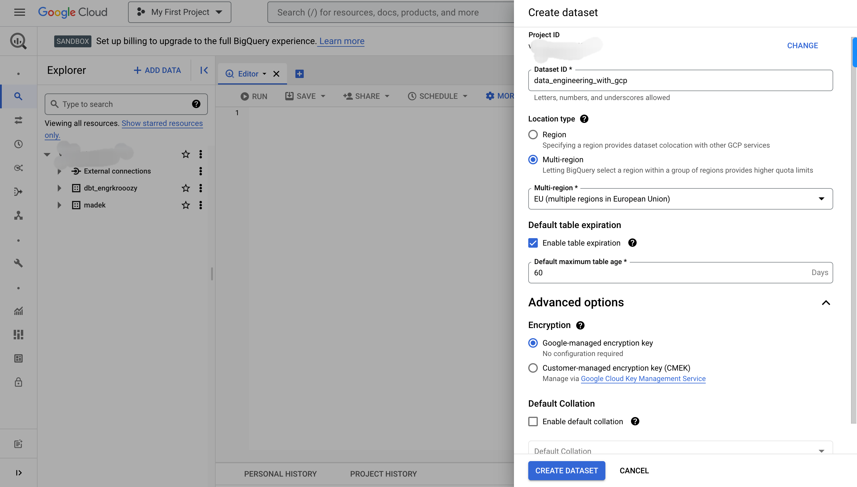
To create a dataset, you have to specify the following information:
A dataset ID: the dataset's name (unique per project)
Data location: dataset's geographical location
Default table expiration: specify a dataset's time to live.
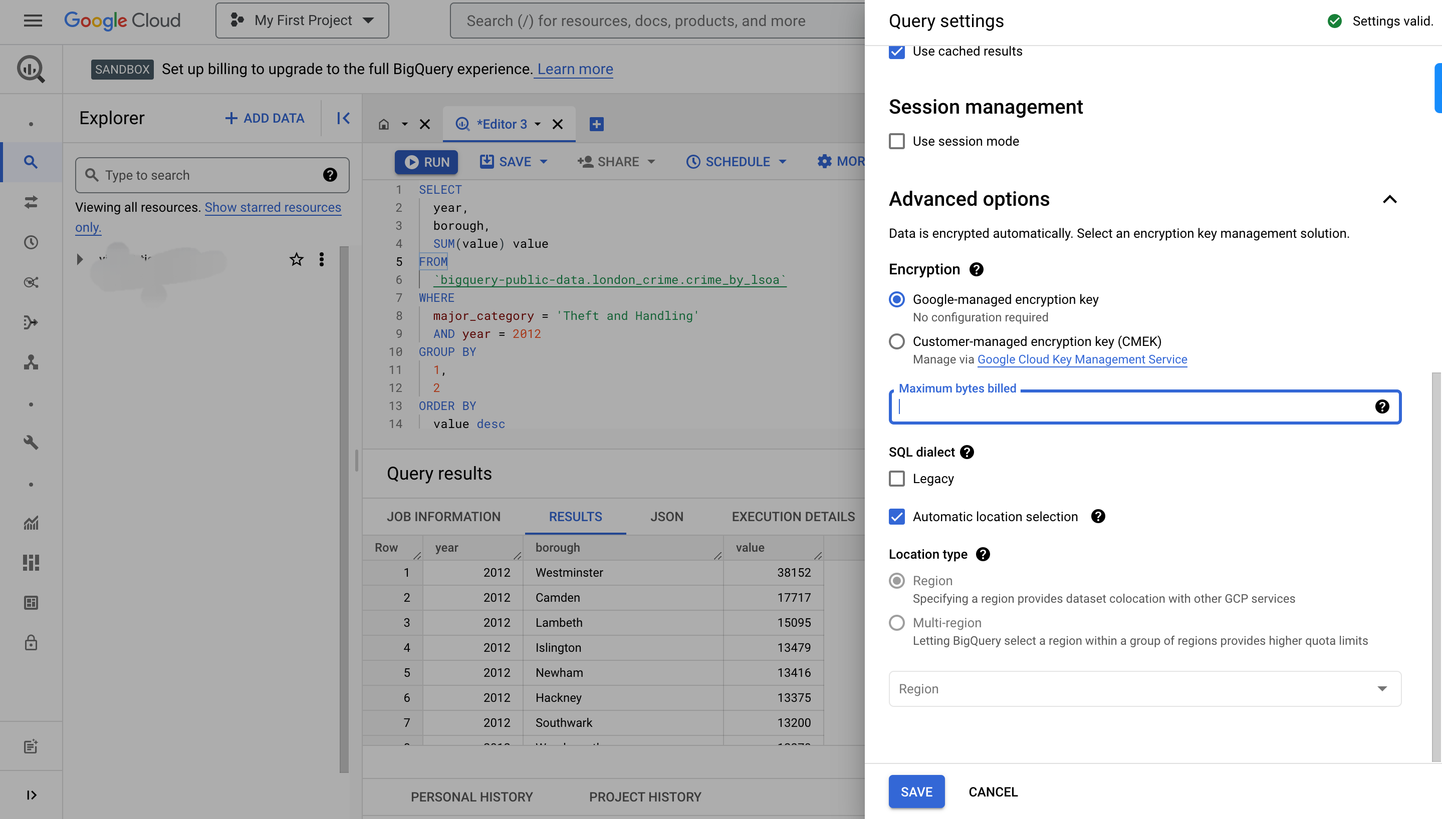
SELECT year, borough, SUM(value) value FROM `bigquery-public-data.london_crime.crime_by_lsoa` WHERE major_category = 'Theft and Handling' AND year = 2012 GROUP BY 1,2 ORDER BY value desc

This query pulls the year, borough, and no of crimes that happened in different boroughs in London from the table crime_by_lsoa. The dataset containing that table is called london_crime and is part of the bigquery-public-data Project. Users should note that the project name, dataset name, and table name are in the order they should appear when supplying a table name. When supplying a table name, backticks are used rather than single quotes.
The example below illustrates how to query a dataset using the bq command line on cloud shell. The table names are in backticks, while the SELECT statement contents contain single quotes.
bq query --use_legacy_sql=false \ 'SELECT year, borough, SUM(value) AS value FROM `bigquery-public-data.london_crime.crime_by_lsoa` WHERE major_category = "Theft and Handling" AND year = 2012 GROUP BY 1,2 ORDER BY value desc'

The bq query command accepts an argument specifying the SQL variant to use while scripting. BigQuery supports two varieties of SQL: legacy and standard. Standard SQL is the preferred variant as it is ANSI compliant. In addition, standard SQL includes sophisticated capabilities such as connected subqueries, ARRAY, STRUCT, JSON data types, and complicated join queries.
BigQuery utilises slots, which are discrete processing units, to process queries. BigQuery determines the number of slots required to perform each query based on size and complexity.
BigQuery offers two price tiers for the time slots used to execute your queries:
On-demand billing: Queries use a shared pool of slots and are charged for the number of bytes processed.
Flat-rate billing: Buy dedicated slot capacity to run queries for a fixed price.
Data Exporting and Loading
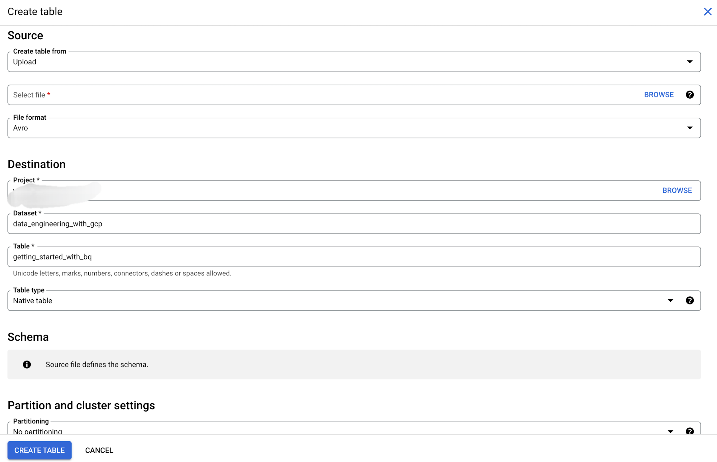
You can make tables with an existing dataset and load data into them. There are numerous methods for ingesting data into BigQuery among them are:
Loading data records in batches.
Stream a single record or several records at once.
Create new data using queries, then add or replace the results in a table.
Batch Loads
Using batch loading, you load the source data into a BigQuery database at once. A CSV file, an external database, or a collection of log files might be used as data sources.
Batch loading can be done at once or regularly using orchestration services like Airflow (Cloud Composer), cron jobs or BigQuery Data Transfer Service.
The following are some choices for batch loading in BigQuery:
Load Jobs: Load data from Cloud Storage or local files in Avro, CSV, JSON, ORC, or Parquet formats.
SQL: LOAD DATA SQL statement loads data from files into tables.
BigQuery Data Transfer Service: Automate data loading from Google SaaS and third-party applications.
BigQuery Storage Write API: batch-process data and load them in a single atomic action.

Streaming
Streaming involves sending smaller chunks of data in real-time, allowing for data querying as they arrive. The following are some of the BigQuery streaming options:
Storage Write API: High-throughput streaming ingestion with exactly-once delivery.
Dataflow: Use a Dataflow streaming pipeline to write to BigQuery.
BigQuery Connector for SAP: close to real-time replication of SAP data into BigQuery.
Create New Data Using Queries
Data in BigQuery tables may be created from SQL queries. Creating new data includes:
DML commands can insert data in bulk and save query results.
To create a new table from a query result, use CREATE TABLE... AS.
Execute a query and store the results in a table.
Clustering, Partitioning, and Sharding
BigQuery supports the creation of clustered tables. Data in clustered tables are automatically grouped depending on one or more column contents.
A clustered table contains data that are related to one another. This arrangement could increase the speed of some queries, particularly those that filter rows using the columns used to cluster data. You can also partition on clustered tables.
Huge tables should be divided into smaller ones or partitioned to increase query efficiency. For example, partitions can separate data by date or timestamp, while sharding can break data into several tables based on other criteria using a naming prefix such as [PREFIX]_YYYYMMDD.
Tables with partitions perform better than tables that are sharded. BigQuery must keep a copy of each table's metadata and schema when sharding. Permissions for each table being queried by BigQuery also need to be checked. This technique also increases the query burden and negatively affects query speed.
Monitoring and Logging in BigQuery
BigQuery uses Cloud Monitoring and Cloud Audit Logs for monitoring and logging. The performance indicators offered by cloud monitoring include query counts and execution times. In addition, to keep track of activities like task execution and table creation, one can utilise Cloud Audit Logs.
With cloud Monitoring, you can configure dashboards to observe critical metrics like the number of jobs running, how many bytes were scanned during a query, and the distribution of query times.

Cloud Logging tracks event log entries such as Inserting, updating and deleting tables, jobs and Executing queries.
Monitoring helps learn how your queries and tasks are functioning, whereas logs are helpful for learning who is acting in BigQuery.

BigQuery Cost Considerations
BigQuery rates vary depending on how much data is read, stored or streamed. Visit the pricing page to view the current rates.
Before executing a query, you may use one of the following ways to estimate costs: Google Cloud console query validator, Google Cloud pricing calculator, --dry_run flag in the bq command line.
BigQuery Best Practices
Here are some rules of thumb to follow to maximise BigQuery performance and optimise cost:
Examine data with preview options: Do not execute queries to examine or inspect table data.
Limit query costs by restricting bytes: To reduce query costs, specify the maximum bytes billed value.
Refrain from SELECT *: Just the needed columns should be queried.
Price your queries before executing them: Check the charges of your queries before executing them.
Use clustered or partitioned tables: To decrease the quantity of data examined, use clustering and partitioning.
Avoid using LIMIT to minimise expenses in non-clustered tables: Using a LIMIT clause does not reduce costs for non-clustered tables.